- 空的DataFrame中插入数据
Pandas reference links
http://pandas.pydata.org/pandas-docs/stable/
http://pandas.pydata.org/pandas-docs/stable/api.html
http://www.cnblogs.com/chaosimple/p/4153083.html
http://www.shizhuolin.com/2015/04/19/978.html
https://ericfu.me/10-minutes-to-pandas/
http://blog.csdn.net/xiaodongxiexie/article/details/53108959
http://blog.csdn.net/wr339988/article/details/65446138
Pandas进阶
http://dataunion.org/23394.html
http://cloga.info/python/%E6%95%B0%E6%8D%AE%E7%A7%91%E5%AD%A6/2013/09/17/pandasintro
http://www.jianshu.com/p/682c24aef525
https://www.joinquant.com/post/1198
https://wolfsonliu.github.io/archive/python-xue-xi-bi-ji-pandas.html
https://stream886.github.io/2016/12/18/%E6%95%B0%E6%8D%AE%E5%88%86%E6%9E%90%E5%B8%B8%E7%94%A8%E6%93%8D%E4%BD%9C%E7%AC%94%E8%AE%B0%E2%80%94%E2%80%94Python%E4%B9%8BPandas%E5%8C%85/
http://xxuan.me/2017-09-28-pandas.html
https://github.com/familyld/learnpython/blob/master/Efficient_Pandas_Skills.md
http://xight.top/2015/10/23/pandas-%E6%8C%87%E5%8D%97-2/
https://zhuanlan.zhihu.com/p/21598982
http://kekefund.com/2016/06/17/pandas-groupby/
DataFrame获取列名
1 | k_df.columns |
DataFrame列作为list返回
1 | list(k_df.columns) |
获取DataFrame中的某个值
1 | code_df.iat[index, 0] # 第一个参数为index值,后一个参数是列所在的索引 |
设置DataFrame中的某个值
1 | df.at[dates[0],'A'] = 0 |
列交换位置
1 | # A list |
取前两列
1 | code_df = today_df[list(today_df.columns[0:2])] |
插入一列
1 | # 第一个参数为插入位置,列名为date,值为today_date_str |
插入一行
1 | low_increase_df = today_df[0:0] |
获取dateFrame的索引值
1 | basics_df.index |
获取某一列或几列的所有值
http://www.cnblogs.com/kylinlin/p/5231404.html
INDEXING AND SELECTING DATA chapter in pandas document
p11931
2
3
4
5
6
7
8
9
10
11
12
13
14
15
16
17
18
19
20
21
22
23
24
25
26
27
28
29
30
31
32df.loc[:,['A','B']]
>>> list(hist_df)
['open', 'high', 'close', 'low', 'volume', 'price_change', 'p_change', 'ma5', 'ma10', 'ma20', 'v_ma5', 'v_ma10', 'v_ma20', 'turnover']
>>> list(hist_df.columns)
['open', 'high', 'close', 'low', 'volume', 'price_change', 'p_change', 'ma5', 'ma10', 'ma20', 'v_ma5', 'v_ma10', 'v_ma20', 'turnover']
>>> hist_df.columns[1]
'high'
>>> hist_df.columns[0]
'open'
>>> len(hist_df.columns)
14
>>> list(hist_df.columns).index('open')
0
>>> list(hist_df.columns).index('low')
3
today_df[:]['code']
today_df[today_df.columns[0]]
today_df.today_df
today_df['code']
today_df[['code', 'name', 'volume']]
today_df[[1, 2, 3, 4, 5, 8]]
today_df.loc[:, list(today_df.columns[0:2])]
today_df.loc[:, 0:2]
pandas revert翻转
today_df = today_df[::-1]
即通过[]获取DataFrame的值,如果只有一个参数或者参数列表,则是获取这些列的值,而且这些参数必须是列名,如:df[['code', 'name', 'volume']], df[df.columns[1:5]]。如果是参数是一个范围,则是获取行的值,如df[0:len(df)-1], df[::2]
复制DataFrame
1 | new_code_df = code_df[:] |
复制DataFrame的结构
1 | new_code_df = code_df[:0] # 复制空的DataFrame |
创建DataFrame
http://blog.csdn.net/chixujohnny/article/details/541338661
2
3
4
5
6
7
8
9
10
11
12
13
14
15
16df = pd.DataFrame(np.random.randn(6,4), index=dates, columns=list('ABCD'))
# 创建一个空的 DataFrame
import pandas as pd
df_empty = pd.DataFrame(columns=['A', 'B', 'C', 'D'])
df = DataFrame(np.random.randn(4, 5), columns=['A', 'B', 'C', 'D', 'E'])
DataFrame数据预览:
A B C D E
0 0.673092 0.230338 -0.171681 0.312303 -0.184813
1 -0.504482 -0.344286 -0.050845 -0.811277 -0.298181
2 0.542788 0.207708 0.651379 -0.656214 0.507595
3 -0.249410 0.131549 -2.198480 -0.437407 1.628228
http://blog.sina.com.cn/s/blog_74cd4a3f0102wn5d.html1
2
3
4
5
6
7
8
9
10
11
12
13
14
15
16
17
18
19
20
21
22
23
24
25
26
27
28
29
30
31
32
33
34
35
36
37
38
39pandas.Series.append method in pandas.pdf
# method 1
>>> select_df = pandas.DataFrame(columns=['code', 'price'])
>>> select_df = select_df.append({'code':'600000', 'price':'12.88'},ignore_index=True)
>>> select_df
code price
0 600000 12.88
>>> select_df = select_df.append({'code':'600399', 'price':'2.88'},ignore_index=True)
>>> select_df
code price
0 600000 12.88
1 600399 2.88
>>> select_df = select_df.append([600123, 15.12],ignore_index=True)
>>> select_df
code price 0
0 600000 12.88 NaN
1 600399 2.88 NaN
2 NaN NaN 600123.00
3 NaN NaN 15.12
# method 2
在pandas中创建一个空DataFrame的方法,类似于创建了一个空字典(dict)。
例如:empty = pandas.DataFrame({"name":"","age":"","sex":""})
想要向empty中插入一行数据,可以用同样的方法。
(1)首先,要创建一个DataFrame。要注意,在这里需加入index属性,new = pandas.DataFrame({"name":"","age":"","sex":""},index=["0"])。
(2)然后,开始插值。ignore_index=True,可以帮助忽略index,自动递增。
empty.append(new,ignore_index=True)
(3)最重要的,赋值给empty.
empty = empty.append(new,ignore_index=True)
否则,数据始终没有写入。
DataFrame数据过滤
http://bluewhale.cc/2016-08-06/use-pandas-filter-and-sort.html
http://www.cnblogs.com/renfanzi/p/6420783.html
http://blog.csdn.net/zhili8866/article/details/681344811
2
3
4
5
6
7
8
9
10
11
12today_trade_df = today_df[today_df.volume > 0]
today_df[today_df.code == '600000'] # 取得code列中数据为600000的行
today_df[today_df['code'] == '600000']
today_df[(today_df['code'] >= '600000') & (today_df['volume'] > 100000)]
price_today_df = today_df[(today_df.trade < 50) & (today_df.trade > 0)]
price_today_df = today_df[(today_df.trade < 50) & (today_df.volume > 0)]
price_today_df.sort_values(by='trade') #升序排列
price_today_df.sort_values(by='trade', ascending=False) #降序排列
price_today_df.sort_values(by=['trade', 'high'], ascending=False) #降序排列,主降序列为trade,次降序列为high
https://stackoverflow.com/questions/14247586/python-pandas-how-to-select-rows-with-one-or-more-nulls-from-a-dataframe-without
https://stackoverflow.com/questions/21202652/getting-all-rows-with-nan-value
https://stackoverflow.com/questions/40245507/python-pandas-selecting-rows-whose-column-value-is-null-none-nan
https://stackoverflow.com/questions/38368490/pandas-dataframe-select-the-specific-columns-with-nan-values
https://stackoverflow.com/questions/22551403/python-pandas-filtering-out-nan-from-a-data-selection-of-a-column-of-strings
https://stackoverflow.com/questions/16017034/to-extract-non-nan-values-from-multiple-rows-in-a-pandas-dataframe1
2
3
4
5
6
7basics_df[pandas.isnull(basics_df['area'])] # 获取area列中值为空(numpy.nan)的行
basics_df[pandas.isnull(basics_df).any(axis=1)] # 获取所有列中值为空(numpy.nan)的行
basics_df[pandas.notnull(basics_df['area'])] # 获取area列中值不为空的行
new_df = basics_df.dropna() # 获取所有列中值不为空的行
new_df = basics_df[basics_df.columns[:4]].dropna() # 获取前四列中值不为空的行
求每列最大值,最小值,和,平均值
http://www.cnblogs.com/wuzhiblog/p/python_new_row_or_col.html1
2
3
4
5
6
7
8
9
10
11
12
13
14
15
16
17
18
19
20
21
22
23
24
25
26
27
28
29
30
31
32
33
34
35
36
37
38
39
40
41
42
43
44
45
46
47
48
49
50
51
52
53
54
55
56
57
58
59
60
61
62
63
64
65
66
67
68
69
70
71
72
73
74
75
76
77
78
79
80
81
82
83
84
85
86
87pandas.pdf P504
>>> dir(price_today_df)
['T', '_AXIS_ALIASES', '_AXIS_IALIASES', '_AXIS_LEN', '_AXIS_NAMES', '_AXIS_NUMBERS', '_AXIS_ORDERS', '_AXIS_REVERSED', '_AXIS_SLICEMAP', '__abs__', '__add__', '__and__', '__array__', '__array_wrap__', '__bool__', '__bytes__', '__class__', '__contains__', '__copy__', '__deepcopy__', '__delattr__', '__delitem__', '__dict__', '__dir__', '__div__', '__doc__', '__eq__', '__finalize__', '__floordiv__', '__format__', '__ge__', '__getattr__', '__getattribute__', '__getitem__', '__getstate__', '__gt__', '__hash__', '__iadd__', '__imul__', '__init__', '__init_subclass__', '__invert__', '__ipow__', '__isub__', '__iter__', '__itruediv__', '__le__', '__len__', '__lt__', '__mod__', '__module__', '__mul__', '__ne__', '__neg__', '__new__', '__nonzero__', '__or__', '__pow__', '__radd__', '__rand__', '__rdiv__', '__reduce__', '__reduce_ex__', '__repr__', '__rfloordiv__', '__rmod__', '__rmul__', '__ror__', '__round__', '__rpow__', '__rsub__', '__rtruediv__', '__rxor__', '__setattr__', '__setitem__', '__setstate__', '__sizeof__', '__str__', '__sub__', '__subclasshook__', '__truediv__', '__unicode__', '__weakref__', '__xor__', '_accessors', '_add_numeric_operations', '_add_series_only_operations', '_add_series_or_dataframe_operations', '_agg_by_level', '_agg_doc', '_aggregate', '_aggregate_multiple_funcs', '_align_frame', '_align_series', '_apply_broadcast', '_apply_empty_result', '_apply_raw', '_apply_standard', '_at', '_box_col_values', '_box_item_values', '_builtin_table', '_check_inplace_setting', '_check_is_chained_assignment_possible', '_check_percentile', '_check_setitem_copy', '_clear_item_cache', '_combine_const', '_combine_frame', '_combine_match_columns', '_combine_match_index', '_combine_series', '_combine_series_infer', '_compare_frame', '_compare_frame_evaluate', '_consolidate', '_consolidate_inplace', '_construct_axes_dict', '_construct_axes_dict_for_slice', '_construct_axes_dict_from', '_construct_axes_from_arguments', '_constructor', '_constructor_expanddim', '_constructor_sliced', '_convert', '_count_level', '_create_indexer', '_cython_table', '_dir_additions', '_dir_deletions', '_ensure_valid_index', '_expand_axes', '_flex_compare_frame', '_from_arrays', '_from_axes', '_get_agg_axis', '_get_axis', '_get_axis_name', '_get_axis_number', '_get_axis_resolvers', '_get_block_manager_axis', '_get_bool_data', '_get_cacher', '_get_index_resolvers', '_get_item_cache', '_get_numeric_data', '_get_values', '_getitem_array', '_getitem_column', '_getitem_frame', '_getitem_multilevel', '_getitem_slice', '_gotitem', '_iat', '_iget_item_cache', '_iloc', '_indexed_same', '_info_axis', '_info_axis_name', '_info_axis_number', '_info_repr', '_init_dict', '_init_mgr', '_init_ndarray', '_internal_names', '_internal_names_set', '_is_builtin_func', '_is_cached', '_is_cython_func', '_is_datelike_mixed_type', '_is_mixed_type', '_is_numeric_mixed_type', '_is_view', '_ix', '_ixs', '_join_compat', '_loc', '_maybe_cache_changed', '_maybe_update_cacher', '_metadata', '_needs_reindex_multi', '_obj_with_exclusions', '_protect_consolidate', '_reduce', '_reindex_axes', '_reindex_axis', '_reindex_columns', '_reindex_index', '_reindex_multi', '_reindex_with_indexers', '_repr_data_resource_', '_repr_fits_horizontal_', '_repr_fits_vertical_', '_repr_html_', '_repr_latex_', '_reset_cache', '_reset_cacher', '_sanitize_column', '_selected_obj', '_selection', '_selection_list', '_selection_name', '_series', '_set_as_cached', '_set_axis', '_set_axis_name', '_set_is_copy', '_set_item', '_setitem_array', '_setitem_frame', '_setitem_slice', '_setup_axes', '_shallow_copy', '_slice', '_stat_axis', '_stat_axis_name', '_stat_axis_number', '_try_aggregate_string_function', '_typ', '_unpickle_frame_compat', '_unpickle_matrix_compat', '_update_inplace', '_validate_dtype', '_values', '_where', '_xs', 'abs', 'add', 'add_prefix', 'add_suffix', 'agg', 'aggregate', 'align', 'all', 'amount', 'any', 'append', 'apply', 'applymap', 'as_blocks', 'as_matrix', 'asfreq', 'asof', 'assign', 'astype', 'at', 'at_time', 'axes', 'between_time', 'bfill', 'blocks', 'bool', 'boxplot', 'changepercent', 'clip', 'clip_lower', 'clip_upper', 'code', 'columns', 'combine', 'combine_first', 'compound', 'consolidate', 'convert_objects', 'copy', 'corr', 'corrwith', 'count', 'cov', 'cummax', 'cummin', 'cumprod', 'cumsum', 'describe', 'diff', 'div', 'divide', 'dot', 'drop', 'drop_duplicates', 'dropna', 'dtypes', 'duplicated', 'empty', 'eq', 'equals', 'eval', 'ewm', 'expanding', 'ffill', 'fillna', 'filter', 'first', 'first_valid_index', 'floordiv', 'from_csv', 'from_dict', 'from_items', 'from_records', 'ftypes', 'ge', 'get', 'get_dtype_counts', 'get_ftype_counts', 'get_value', 'get_values', 'groupby', 'gt', 'head', 'high', 'hist', 'iat', 'idxmax', 'idxmin', 'iloc', 'index', 'info', 'insert', 'interpolate', 'is_copy', 'isin', 'isnull', 'items', 'iteritems', 'iterrows', 'itertuples', 'ix', 'join', 'keys', 'kurt', 'kurtosis', 'last', 'last_valid_index', 'le', 'loc', 'lookup', 'low', 'lt', 'mad', 'mask', 'max', 'mean', 'median', 'melt', 'memory_usage', 'merge', 'min', 'mktcap', 'mod', 'mode', 'mul', 'multiply', 'name', 'ndim', 'ne', 'nlargest', 'nmc', 'notnull', 'nsmallest', 'nunique', 'open', 'pb', 'pct_change', 'per', 'pipe', 'pivot', 'pivot_table', 'plot', 'pop', 'pow', 'prod', 'product', 'quantile', 'query', 'radd', 'rank', 'rdiv', 'reindex', 'reindex_axis', 'reindex_like', 'rename', 'rename_axis', 'reorder_levels', 'replace', 'resample', 'reset_index', 'rfloordiv', 'rmod', 'rmul', 'rolling', 'round', 'rpow', 'rsub', 'rtruediv', 'sample', 'select', 'select_dtypes', 'sem', 'set_axis', 'set_index', 'set_value', 'settlement', 'shape', 'shift', 'size', 'skew', 'slice_shift', 'sort_index', 'sort_values', 'sortlevel', 'squeeze', 'stack', 'std', 'style', 'sub', 'subtract', 'sum', 'swapaxes', 'swaplevel', 'tail', 'take', 'to_clipboard', 'to_csv', 'to_dense', 'to_dict', 'to_excel', 'to_feather', 'to_gbq', 'to_hdf', 'to_html', 'to_json', 'to_latex', 'to_msgpack', 'to_panel', 'to_period', 'to_pickle', 'to_records', 'to_sparse', 'to_sql', 'to_stata', 'to_string', 'to_timestamp', 'to_xarray', 'trade', 'transform', 'transpose', 'truediv', 'truncate', 'tshift', 'turnoverratio', 'tz_convert', 'tz_localize', 'unstack', 'update', 'values', 'var', 'volume', 'where', 'xs']
>>>
>>> dir(pandas.Series)
['T', '_AXIS_ALIASES', '_AXIS_IALIASES', '_AXIS_LEN', '_AXIS_NAMES', '_AXIS_NUMBERS', '_AXIS_ORDERS', '_AXIS_REVERSED', '_AXIS_SLICEMAP', '__abs__', '__add__', '__and__', '__array__', '__array_prepare__', '__array_priority__', '__array_wrap__', '__bool__', '__bytes__', '__class__', '__contains__', '__copy__', '__deepcopy__', '__delattr__', '__delitem__', '__dict__', '__dir__', '__div__', '__divmod__', '__doc__', '__eq__', '__finalize__', '__float__', '__floordiv__', '__format__', '__ge__', '__getattr__', '__getattribute__', '__getitem__', '__getstate__', '__gt__', '__hash__', '__iadd__', '__imul__', '__init__', '__init_subclass__', '__int__', '__invert__', '__ipow__', '__isub__', '__iter__', '__itruediv__', '__le__', '__len__', '__long__', '__lt__', '__mod__', '__module__', '__mul__', '__ne__', '__neg__', '__new__', '__nonzero__', '__or__', '__pow__', '__radd__', '__rand__', '__rdiv__', '__reduce__', '__reduce_ex__', '__repr__', '__rfloordiv__', '__rmod__', '__rmul__', '__ror__', '__round__', '__rpow__', '__rsub__', '__rtruediv__', '__rxor__', '__setattr__', '__setitem__', '__setstate__', '__sizeof__', '__str__', '__sub__', '__subclasshook__', '__truediv__', '__unicode__', '__weakref__', '__xor__', '_accessors', '_add_numeric_operations', '_add_series_only_operations', '_add_series_or_dataframe_operations', '_agg_by_level', '_agg_doc', '_aggregate', '_aggregate_multiple_funcs', '_align_frame', '_align_series', '_allow_index_ops', '_at', '_binop', '_box_item_values', '_builtin_table', '_can_hold_na', '_check_inplace_setting', '_check_is_chained_assignment_possible', '_check_percentile', '_check_setitem_copy', '_clear_item_cache', '_consolidate', '_consolidate_inplace', '_construct_axes_dict', '_construct_axes_dict_for_slice', '_construct_axes_dict_from', '_construct_axes_from_arguments', '_constructor', '_constructor_expanddim', '_constructor_sliced', '_convert', '_create_indexer', '_cython_table', '_dir_additions', '_dir_deletions', '_expand_axes', '_from_axes', '_get_axis', '_get_axis_name', '_get_axis_number', '_get_axis_resolvers', '_get_block_manager_axis', '_get_bool_data', '_get_cacher', '_get_index_resolvers', '_get_item_cache', '_get_numeric_data', '_get_values', '_get_values_tuple', '_get_with', '_gotitem', '_iat', '_iget_item_cache', '_iloc', '_index', '_indexed_same', '_info_axis', '_info_axis_name', '_info_axis_number', '_init_mgr', '_internal_names', '_internal_names_set', '_is_builtin_func', '_is_cached', '_is_cython_func', '_is_datelike_mixed_type', '_is_mixed_type', '_is_numeric_mixed_type', '_is_view', '_ix', '_ixs', '_loc', '_make_cat_accessor', '_make_dt_accessor', '_make_str_accessor', '_maybe_cache_changed', '_maybe_update_cacher', '_metadata', '_needs_reindex_multi', '_obj_with_exclusions', '_protect_consolidate', '_reduce', '_reindex_axes', '_reindex_axis', '_reindex_indexer', '_reindex_multi', '_reindex_with_indexers', '_repr_data_resource_', '_reset_cache', '_reset_cacher', '_selected_obj', '_selection', '_selection_list', '_selection_name', '_set_as_cached', '_set_axis', '_set_axis_name', '_set_is_copy', '_set_item', '_set_labels', '_set_name', '_set_subtyp', '_set_values', '_set_with', '_set_with_engine', '_setup_axes', '_shallow_copy', '_slice', '_stat_axis', '_stat_axis_name', '_stat_axis_number', '_try_aggregate_string_function', '_typ', '_unpickle_series_compat', '_update_inplace', '_validate_dtype', '_values', '_where', '_xs', 'abs', 'add', 'add_prefix', 'add_suffix', 'agg', 'aggregate', 'align', 'all', 'any', 'append', 'apply', 'argmax', 'argmin', 'argsort', 'as_blocks', 'as_matrix', 'asfreq', 'asobject', 'asof', 'astype', 'at', 'at_time', 'autocorr', 'axes', 'base', 'between', 'between_time', 'bfill', 'blocks', 'bool', 'cat', 'clip', 'clip_lower', 'clip_upper', 'combine', 'combine_first', 'compound', 'compress', 'consolidate', 'convert_objects', 'copy', 'corr', 'count', 'cov', 'cummax', 'cummin', 'cumprod', 'cumsum', 'data', 'describe', 'diff', 'div', 'divide', 'dot', 'drop', 'drop_duplicates', 'dropna', 'dt', 'dtype', 'dtypes', 'duplicated', 'empty', 'eq', 'equals', 'ewm', 'expanding', 'factorize', 'ffill', 'fillna', 'filter', 'first', 'first_valid_index', 'flags', 'floordiv', 'from_array', 'from_csv', 'ftype', 'ftypes', 'ge', 'get', 'get_dtype_counts', 'get_ftype_counts', 'get_value', 'get_values', 'groupby', 'gt', 'hasnans', 'head', 'hist', 'iat', 'idxmax', 'idxmin', 'iloc', 'imag', 'index', 'interpolate', 'is_copy', 'is_monotonic', 'is_monotonic_decreasing', 'is_monotonic_increasing', 'is_unique', 'isin', 'isnull', 'item', 'items', 'itemsize', 'iteritems', 'ix', 'keys', 'kurt', 'kurtosis', 'last', 'last_valid_index', 'le', 'loc', 'lt', 'mad', 'map', 'mask', 'max', 'mean', 'median', 'memory_usage', 'min', 'mod', 'mode', 'mul', 'multiply', 'name', 'nbytes', 'ndim', 'ne', 'nlargest', 'nonzero', 'notnull', 'nsmallest', 'nunique', 'pct_change', 'pipe', 'plot', 'pop', 'pow', 'prod', 'product', 'ptp', 'put', 'quantile', 'radd', 'rank', 'ravel', 'rdiv', 'real', 'reindex', 'reindex_axis', 'reindex_like', 'rename', 'rename_axis', 'reorder_levels', 'repeat', 'replace', 'resample', 'reset_index', 'reshape', 'rfloordiv', 'rmod', 'rmul', 'rolling', 'round', 'rpow', 'rsub', 'rtruediv', 'sample', 'searchsorted', 'select', 'sem', 'set_axis', 'set_value', 'shape', 'shift', 'size', 'skew', 'slice_shift', 'sort_index', 'sort_values', 'sortlevel', 'squeeze', 'std', 'str', 'strides', 'sub', 'subtract', 'sum', 'swapaxes', 'swaplevel', 'tail', 'take', 'to_clipboard', 'to_csv', 'to_dense', 'to_dict', 'to_excel', 'to_frame', 'to_hdf', 'to_json', 'to_msgpack', 'to_period', 'to_pickle', 'to_sparse', 'to_sql', 'to_string', 'to_timestamp', 'to_xarray', 'tolist', 'transform', 'transpose', 'truediv', 'truncate', 'tshift', 'tz_convert', 'tz_localize', 'unique', 'unstack', 'update', 'valid', 'value_counts', 'values', 'var', 'view', 'where', 'xs']
>>>
>>> price_today_df['open'].min()
2.2999999999999998
>>> price_today_df['open'].max()
44.899999999999999
>>> price_today_df['open'].sum()
908.0200000000001
>>> price_today_df['open'].mean() # 平均值
12.106933333333334
>>>
decribe方法可以计算各个列的基本描述统计值。包含计数,平均数,标准差,最大值,最小值及4分位差。
>>> price_today_df.describe()
changepercent trade open high low settlement \
count 75.000000 75.000000 75.000000 75.000000 75.000000 75.000000
mean -0.145907 12.080800 12.106933 12.197200 11.999200 12.116667
std 1.045732 8.322333 8.365313 8.419518 8.254416 8.386995
min -4.398000 2.310000 2.300000 2.330000 2.290000 2.300000
25% -0.515000 6.700000 6.720000 6.755000 6.695000 6.720000
50% -0.180000 9.700000 9.690000 9.760000 9.610000 9.680000
75% 0.285000 14.830000 15.145000 15.170000 14.810000 15.135000
max 3.141000 45.220000 44.900000 45.450000 44.540000 44.970000
volume turnoverratio amount per pb \
count 7.500000e+01 75.000000 7.500000e+01 75.000000 75.000000
mean 1.600905e+07 0.320844 1.488266e+08 104.235147 2.710467
std 3.957963e+07 0.275348 3.324918e+08 288.945301 9.484397
min 2.493000e+05 0.029590 4.033473e+06 -199.625000 0.000000
25% 1.375174e+06 0.141150 1.267183e+07 12.444500 0.000000
50% 3.410731e+06 0.205090 2.308137e+07 22.996000 1.403000
75% 9.177329e+06 0.475250 1.029047e+08 47.775500 2.500000
max 2.798431e+08 1.320230 2.179901e+09 1512.308000 81.917000
mktcap nmc
count 7.500000e+01 7.500000e+01
mean 5.594753e+06 4.700628e+06
std 1.217174e+07 9.934420e+06
min 2.554133e+05 2.251359e+05
25% 8.680703e+05 6.782128e+05
50% 1.441800e+06 1.325663e+06
75% 4.347619e+06 3.365268e+06
max 7.336915e+07 5.790801e+07
>>>
http://www.cnblogs.com/wuzhiblog/p/python_new_row_or_col.html
导入模块:
from pandas import DataFrame
import pandas as pd
import numpy as np
生成DataFrame数据
df = DataFrame(np.random.randn(4, 5), columns=['A', 'B', 'C', 'D', 'E'])
DataFrame数据预览:
A B C D E
0 0.673092 0.230338 -0.171681 0.312303 -0.184813
1 -0.504482 -0.344286 -0.050845 -0.811277 -0.298181
2 0.542788 0.207708 0.651379 -0.656214 0.507595
3 -0.249410 0.131549 -2.198480 -0.437407 1.628228
计算各列数据总和并作为新列添加到末尾
df['Col_sum'] = df.apply(lambda x: x.sum(), axis=1)
计算各行数据总和并作为新行添加到末尾
df.loc['Row_sum'] = df.apply(lambda x: x.sum())
最终数据结果:
A B C D E Col_sum
0 0.673092 0.230338 -0.171681 0.312303 -0.184813 0.859238
1 -0.504482 -0.344286 -0.050845 -0.811277 -0.298181 -2.009071
2 0.542788 0.207708 0.651379 -0.656214 0.507595 1.253256
3 -0.249410 0.131549 -2.198480 -0.437407 1.628228 -1.125520
Row_sum 0.461987 0.225310 -1.769627 -1.592595 1.652828 -1.022097
判断某列是否有空值
https://stackoverflow.com/questions/29530232/how-to-check-if-any-value-is-nan-in-a-pandas-dataframe
https://blog.csdn.net/cc_jjj/article/details/78879839
https://blog.csdn.net/Guo_ya_nan/article/details/81013510
9.4.4 Boolean Reductions(pandas.v0.23.4.pdf, P596)
You can apply the reductions: empty, any(), all(), and bool() to provide a way to summarize a boolean result.1
2
3
4
5
6
7
8
9
10
11
12
13
14
15
16
17
18
19
20
21
22
23
24
25
26
27
28
29
30
31
32
33
34
35
36
37
38
39
40
41
42
43
44
45
46
47
48
49
50
51
52
53
54
55
56
57
58
59
60
61
62
63
64
65
66
67
68
69
70
71
72
73
74
75
76
77
78
79
80
81
82
83
84
85
86
87
88
89
90
91
92
93
94
95
96
97
98
99
100
101
102
103
104
105
106
107
108
109
110
111
112
113
114
115
116
117
118
119
120
121
122import tushare as ts
import pandas
k_df = ts.get_k_data('600000')
k_df = k_df.tail(10)
k_df_column = list(k_df)
k_df_column.insert(0, k_df_column.pop(k_df_column.index(k_df.columns[-1]))) # 把最后一行弹出插入第一行
k_df = k_df[k_df_column]
k_df['price_change'] = k_df['close'].diff()
k_df['p_change'] = k_df['close'].pct_change() * 100
print(k_df)
ma_list = [5, 10, 20, 60, 250]
# 移动平均数
for ma in ma_list:
k_df['ma' + str(ma)] = k_df['close'].rolling(ma).mean()
# 移动平均数
for ma in ma_list:
k_df['v_ma' + str(ma)] = k_df['volume'].rolling(ma).mean()
print(k_df)
# 判断是否有空值的行
# print(pandas.isnull(k_df))
# print(k_df.isna())
# print(k_df[k_df.isnull().values==True])
print(k_df['code'].notnull().all())
print(k_df.isna().any())
print(k_df.isna().any().any())
print(k_df.isnull().any().any())
print(k_df.isnull().sum().any())
print(k_df.isnull().any().sum()) # 空行的数目
Output:
code date open close high low volume price_change \
631 600000 2018-11-28 10.56 10.58 10.62 10.50 183396.0 NaN
632 600000 2018-11-29 10.64 10.63 10.75 10.54 206856.0 0.05
633 600000 2018-11-30 10.65 10.71 10.75 10.62 285726.0 0.08
634 600000 2018-12-03 10.99 11.02 11.05 10.84 430490.0 0.31
635 600000 2018-12-04 11.00 11.08 11.08 10.97 208112.0 0.06
636 600000 2018-12-05 10.99 11.00 11.10 10.96 254912.0 -0.08
637 600000 2018-12-06 10.82 10.90 10.93 10.82 235979.0 -0.10
638 600000 2018-12-07 10.94 10.89 11.03 10.88 105805.0 -0.01
639 600000 2018-12-10 10.77 10.83 10.90 10.77 159275.0 -0.06
640 600000 2018-12-11 10.84 10.73 10.90 10.69 153033.0 -0.10
p_change
631 NaN
632 0.472590
633 0.752587
634 2.894491
635 0.544465
636 -0.722022
637 -0.909091
638 -0.091743
639 -0.550964
640 -0.923361
code date open close high low volume price_change \
631 600000 2018-11-28 10.56 10.58 10.62 10.50 183396.0 NaN
632 600000 2018-11-29 10.64 10.63 10.75 10.54 206856.0 0.05
633 600000 2018-11-30 10.65 10.71 10.75 10.62 285726.0 0.08
634 600000 2018-12-03 10.99 11.02 11.05 10.84 430490.0 0.31
635 600000 2018-12-04 11.00 11.08 11.08 10.97 208112.0 0.06
636 600000 2018-12-05 10.99 11.00 11.10 10.96 254912.0 -0.08
637 600000 2018-12-06 10.82 10.90 10.93 10.82 235979.0 -0.10
638 600000 2018-12-07 10.94 10.89 11.03 10.88 105805.0 -0.01
639 600000 2018-12-10 10.77 10.83 10.90 10.77 159275.0 -0.06
640 600000 2018-12-11 10.84 10.73 10.90 10.69 153033.0 -0.10
p_change ma5 ma10 ma20 ma60 ma250 v_ma5 v_ma10 v_ma20 \
631 NaN NaN NaN NaN NaN NaN NaN NaN NaN
632 0.472590 NaN NaN NaN NaN NaN NaN NaN NaN
633 0.752587 NaN NaN NaN NaN NaN NaN NaN NaN
634 2.894491 NaN NaN NaN NaN NaN NaN NaN NaN
635 0.544465 10.804 NaN NaN NaN NaN 262916.0 NaN NaN
636 -0.722022 10.888 NaN NaN NaN NaN 277219.2 NaN NaN
637 -0.909091 10.942 NaN NaN NaN NaN 283043.8 NaN NaN
638 -0.091743 10.978 NaN NaN NaN NaN 247059.6 NaN NaN
639 -0.550964 10.940 NaN NaN NaN NaN 192816.6 NaN NaN
640 -0.923361 10.870 10.837 NaN NaN NaN 181800.8 222358.4 NaN
v_ma60 v_ma250
631 NaN NaN
632 NaN NaN
633 NaN NaN
634 NaN NaN
635 NaN NaN
636 NaN NaN
637 NaN NaN
638 NaN NaN
639 NaN NaN
640 NaN NaN
True
code False
date False
open False
close False
high False
low False
volume False
price_change True
p_change True
ma5 True
ma10 True
ma20 True
ma60 True
ma250 True
v_ma5 True
v_ma10 True
v_ma20 True
v_ma60 True
v_ma250 True
dtype: bool
True
True
True
12
空值填充
1 | df.dropna() # 删除含有空值的行或列 |
获取某一行的值
https://pandas.pydata.org/pandas-docs/stable/indexing.html
https://stackoverflow.com/questions/28757389/loc-vs-iloc-vs-ix-vs-at-vs-iat
http://blog.csdn.net/xw_classmate/article/details/51333646
http://blog.csdn.net/wr339988/article/details/65446138
https://www.zhihu.com/question/47362048
http://blog.csdn.net/IAlexanderI/article/details/70186801
http://www.cnblogs.com/coskaka/p/6107372.html
loc: only work on index
iloc: work on position
ix: You can get data from dataframe without it being in the index
at: get scalar values. It’s a very fast loc
iat: Get scalar values. It’s a very fast iloc
http://www.cnblogs.com/kylinlin/p/5231404.html
从如下示例可以看出,loc和iloc在某些情况下可以混用(即行索引为数字的时候),而且iloc支持-1等索引值(位置可以是-1),但是iloc不包括列表的最后一行。loc通过行标签索引行数据,loc[index]这个index是DataFrame的索引,可以是数字,日期或者其它格式索引。iloc通过行号获取行数据,iloc[index]中,这个index是行号,永远是数字。
at的使用方法与loc类似,但是比loc有更快的访问数据的速度,而且只能访问单个元素,不能访问多个元素。
iat对于iloc的关系就像at对于loc的关系,是一种更快的基于索引位置的选择方法,同at一样只能访问单个元素。
http://www.cnblogs.com/harvey888/p/6006200.html
http://blog.csdn.net/wr339988/article/details/65446138
ix,以上说过的几种方法都要求查询的值在索引中,或者位置不超过长度范围,而ix允许你得到不在DataFrame索引中的数据。1
2
3
4
5
6
7
8
9
10
11
12
13
14
15
16
17
18
19
20
21
22
23
24
25
26
27
28
29
30
31
32
33
34
35
36
37# 第一行的值
today_df.head(1)
today_df[:1]
today_df[0:1]
today_df.loc[0]
today_df.iloc[0]
# 前5行的值
today_df[0:5]
today_df.loc[0:4]
today_df.iloc[0:5]
today_df.head()
# 最后一行的值
today_df.tail(1)
today_df[-1:len(today_df)]
today_df.loc[len(today_df) - 1]
today_df.iloc[-1]
# 最后5行的值
today_df[-5:len(today_df)]
today_df.loc[len(today_df) - 5: len(today_df)]
today_df.iloc[-5:len(today_df)]
today_df.tail()
# 获取前五行,只包含前两列的DataFrame
today_df[:5][['code', 'name']]
today_df[:5][today_df.columns[0:2]]
today_df.loc[0:4, list(today_df.columns[0:2])]
today_df.iloc[0:5, 0:2]
today_df.loc[[1,2,4], :]
today_df.iloc[[1,2,4], :]
today_df.loc[[1,2,4]]
today_df.iloc[[1,2,4]]
today_df.loc[[1,2,4], [today_df.columns[0], today_df.columns[2]]]
today_df.iloc[[1,2,4], [0, 2]]
Pandas中loc ,iloc,ix,iat区别
http://www.cnblogs.com/coskaka/p/6107372.html
https://stackoverflow.com/questions/28757389/loc-vs-iloc-vs-ix-vs-at-vs-iat
http://www.cnblogs.com/harvey888/p/6006200.html
http://chnwentao.com/2016/05/24/cix1k7nbv005c2q1p1bk2wr4d/
http://www.shizhuolin.com/2015/04/19/978.html1
2
3
4
5
6
7
8
9
10
11
12
13
14
15
16
17
18
19
20
21
22
23
24
25
26
27
28
29
30
31
32
33
34
35
36
37
38
39
40
41
42
43
44
45
46
47
48
49
50
51
52
53
54
55
56pandas中Loc vs. iloc vs. ix vs. at vs. iat?
所以loc和iloc不能混用,loc是基于index的数值访问(即loc的第一个参数是pandas数据的index),如果index是数字类型,但是不连续,访问的结果与iloc不同,如果index是date或者其它数字类型,则需要用index的数值来访问。而iloc是基于position的数值访问,所以访问的时候不需要去考虑index的值,只需要按照第一行,第几列的方式访问即可。
http://blog.csdn.net/xw_classmate/article/details/51333646
http://blog.csdn.net/wr339988/article/details/65446138
loc: only work on index
loc可以让你按照索引来进行行列选择。
iloc: work on position
如果说loc是按照索引(index)的值来选取的话,那么iloc就是按照索引的位置来进行选取。iloc不关心索引的具体值是多少,只关心位置是多少,所以使用iloc时方括号中只能使用数值。
ix: You can get data from dataframe without it being in the index
以上说过的几种方法都要求查询的秩在索引中,或者位置不超过长度范围,而ix允许你得到不在DataFrame索引中的数据。
ix结合前两种的混合索引,可通过行号索引,也可通过行标签索引
.ix 的功能就更强大了,它允许我们混合使用下标和名称进行选取。 可以说它涵盖了前面所有的用法。基本上把前面的都换成df.ix 都能成功,但是有一点,就是 df.ix [ [ ..1.. ], [..2..] ], 1框内必须统一,必须同时是下标或者名称,2框也一样。
at: get scalar values. It's a very fast loc
at的使用方法与loc类似,但是比loc有更快的访问数据的速度,而且只能访问单个元素,不能访问多个元素。
iat: Get scalar values. It's a very fast iloc
iat对于iloc的关系就像at对于loc的关系,是一种更快的基于索引位置的选择方法,同at一样只能访问单个元素。
>>> df = pd.DataFrame(np.random.randn(10,4), index=range(5,15), columns=list('ABCD'))
>>> df
A B C D
5 -0.319518 0.284740 1.026313 0.431706
6 -0.022680 0.628817 -1.488491 0.149373
7 1.572724 0.566957 1.017841 0.369798
8 -1.143665 0.486865 1.203490 0.118623
9 -0.772590 1.754274 -0.581362 -1.881532
10 -0.233140 0.265633 0.392860 -0.182572
11 0.199502 2.954638 0.506847 -0.295944
12 0.703443 -1.780971 1.181585 2.018214
13 0.648979 0.817560 0.083627 -0.440836
14 -0.025313 -0.823509 1.055526 -0.850109
>>> df.ix[5]
A -0.319518
B 0.284740
C 1.026313
D 0.431706
Name: 5, dtype: float64
>>> df.ix[10]
A -0.233140
B 0.265633
C 0.392860
D -0.182572
Name: 10, dtype: float64
>>> df.ix[9]
A -0.772590
B 1.754274
C -0.581362
D -1.881532
Name: 9, dtype: float64
>>> df.ix[2]
Traceback (most recent call last):
DataFrame排序
1 | # 按照index排序 |
Merge操作
pandas.v0.19.2 p410, p449, p727
http://freefarm.cc/2016/05/24/PANDAS%E5%B8%B8%E7%94%A8%E6%89%8B%E5%86%8C-IV-%E5%90%88%E5%B9%B6%E6%95%B0%E6%8D%AE%E9%9B%86/
https://amaozhao.gitbooks.io/pandas-notebook/content/%E5%90%88%E5%B9%B6%E6%95%B0%E6%8D%AE%E9%9B%86.html
https://www.jianshu.com/p/b07bc5c650ea
https://www.jianshu.com/p/3ec0ca76572b
http://blog.csdn.net/zutsoft/article/details/51498026
http://noahsnail.com/2017/04/29/2017-4-29-pandas%E7%9A%84%E5%9F%BA%E6%9C%AC%E7%94%A8%E6%B3%95(%E5%85%AD)%E2%80%94%E2%80%94%E5%90%88%E5%B9%B6%E6%95%B0%E6%8D%AE/
http://noahsnail.com/2017/04/29/2017-4-29-pandas%E7%9A%84%E5%9F%BA%E6%9C%AC%E7%94%A8%E6%B3%95(%E4%B8%83)%E2%80%94%E2%80%94%E5%90%88%E5%B9%B6%E6%95%B0%E6%8D%AEmerge/
https://morvanzhou.github.io/tutorials/data-manipulation/np-pd/3-6-pd-concat/1
2
3
4
5
6
7
8
9
10
11
12
13
14
15
16
17
18
19
20
21
22
23
24
25
26
27
28
29
30
31
32
33
34
35
36
37
38
39
40
41
42
43
44
45
46
47
48
49
50
51
52
53
54
55
56
57
58
59
60
61
62
63
64
65
66
67
68
69
70
71
72
73
74
75
76
77
78
79
80
81
82
83
84
85
86
87
88
89
90
91
92
93
94
95
96
97
98
99
100
101
102
103
104
105
106
107
108
109
110
111
112
113
114
115
116
117
118
119
120
121
122
123
124
125
126
127
128
129
130
131
132
133
134
135
136
137
138
139
140
141
142
143
144
145
146
147
148
149
150
151
152
153
154
155
156
157
158
1591. concat(注意索引变化)
import pandas as pd
import numpy as np
df = pd.DataFrame(np.random.randn(10, 4))
pieces = [df[:3], df[3:7], df[7:]]
pd.concat(pieces)
pd.concat([df[:3], df[3:7], df[7:]])
>>> df1 = pandas.DataFrame(np.random.randn(6,4), columns=list('ABCD'))
>>> df1
A B C D
0 -1.517306 -0.813150 0.834830 0.998925
1 0.385413 0.281785 -0.213931 -0.321473
2 -0.314647 0.709807 0.849917 1.094283
3 0.453020 -0.264532 1.107129 0.810168
4 0.941546 -0.354594 0.713501 -0.414387
5 -0.299815 -0.706964 -0.694722 0.496755
>>> df2 = pandas.DataFrame(np.random.randn(6,4), columns=list('ABCD'))
>>> df2
A B C D
0 1.248222 -0.032582 -0.410138 0.678771
1 1.491609 0.767659 0.120715 -1.562305
2 -0.648467 -0.746283 -0.160937 -1.644596
3 -1.211631 0.328242 -1.795474 -1.112462
4 1.017662 -0.055081 0.593488 -0.235510
5 -0.423520 0.458304 -0.221281 -0.381890
>>> df_concat = pandas.concat([df1, df2])
>>> df_concat
A B C D
0 -1.517306 -0.813150 0.834830 0.998925
1 0.385413 0.281785 -0.213931 -0.321473
2 -0.314647 0.709807 0.849917 1.094283
3 0.453020 -0.264532 1.107129 0.810168
4 0.941546 -0.354594 0.713501 -0.414387
5 -0.299815 -0.706964 -0.694722 0.496755
0 1.248222 -0.032582 -0.410138 0.678771
1 1.491609 0.767659 0.120715 -1.562305
2 -0.648467 -0.746283 -0.160937 -1.644596
3 -1.211631 0.328242 -1.795474 -1.112462
4 1.017662 -0.055081 0.593488 -0.235510
5 -0.423520 0.458304 -0.221281 -0.381890
>>> df_concat = pandas.concat([df1, df2], ignore_index=True)
>>> df_concat
A B C D
0 -1.517306 -0.813150 0.834830 0.998925
1 0.385413 0.281785 -0.213931 -0.321473
2 -0.314647 0.709807 0.849917 1.094283
3 0.453020 -0.264532 1.107129 0.810168
4 0.941546 -0.354594 0.713501 -0.414387
5 -0.299815 -0.706964 -0.694722 0.496755
6 1.248222 -0.032582 -0.410138 0.678771
7 1.491609 0.767659 0.120715 -1.562305
8 -0.648467 -0.746283 -0.160937 -1.644596
9 -1.211631 0.328242 -1.795474 -1.112462
10 1.017662 -0.055081 0.593488 -0.235510
11 -0.423520 0.458304 -0.221281 -0.381890
2. join
pandas.v0.19.2 p739
https://coolshell.cn/articles/3463.html
http://www.w3school.com.cn/sql/sql_join.asp
3. append(注意索引变化)
less_df = today_df[0:0]
less_df = less_df.append(today_df.iloc[index])
>>> df1 = pandas.DataFrame(np.random.randn(6,4), columns=list('ABCD'))
>>> df1
A B C D
0 -1.517306 -0.813150 0.834830 0.998925
1 0.385413 0.281785 -0.213931 -0.321473
2 -0.314647 0.709807 0.849917 1.094283
3 0.453020 -0.264532 1.107129 0.810168
4 0.941546 -0.354594 0.713501 -0.414387
5 -0.299815 -0.706964 -0.694722 0.496755
>>> df2 = pandas.DataFrame(np.random.randn(6,4), columns=list('ABCD'))
>>> df2
A B C D
0 1.248222 -0.032582 -0.410138 0.678771
1 1.491609 0.767659 0.120715 -1.562305
2 -0.648467 -0.746283 -0.160937 -1.644596
3 -1.211631 0.328242 -1.795474 -1.112462
4 1.017662 -0.055081 0.593488 -0.235510
5 -0.423520 0.458304 -0.221281 -0.381890
>>> df_append = df1.append(df2)
>>> df_append
A B C D
0 -1.517306 -0.813150 0.834830 0.998925
1 0.385413 0.281785 -0.213931 -0.321473
2 -0.314647 0.709807 0.849917 1.094283
3 0.453020 -0.264532 1.107129 0.810168
4 0.941546 -0.354594 0.713501 -0.414387
5 -0.299815 -0.706964 -0.694722 0.496755
0 1.248222 -0.032582 -0.410138 0.678771
1 1.491609 0.767659 0.120715 -1.562305
2 -0.648467 -0.746283 -0.160937 -1.644596
3 -1.211631 0.328242 -1.795474 -1.112462
4 1.017662 -0.055081 0.593488 -0.235510
5 -0.423520 0.458304 -0.221281 -0.381890
>>> df_append = df1.append(df2, ignore_index=True)
>>> df_append
A B C D
0 -1.517306 -0.813150 0.834830 0.998925
1 0.385413 0.281785 -0.213931 -0.321473
2 -0.314647 0.709807 0.849917 1.094283
3 0.453020 -0.264532 1.107129 0.810168
4 0.941546 -0.354594 0.713501 -0.414387
5 -0.299815 -0.706964 -0.694722 0.496755
6 1.248222 -0.032582 -0.410138 0.678771
7 1.491609 0.767659 0.120715 -1.562305
8 -0.648467 -0.746283 -0.160937 -1.644596
9 -1.211631 0.328242 -1.795474 -1.112462
10 1.017662 -0.055081 0.593488 -0.235510
11 -0.423520 0.458304 -0.221281 -0.381890
4. merge
>>> import pandas
>>> import numpy as np
>>> df1 = pandas.DataFrame(np.random.randn(6,4), columns=list('ABCD'))
>>> df1
A B C D
0 -1.517306 -0.813150 0.834830 0.998925
1 0.385413 0.281785 -0.213931 -0.321473
2 -0.314647 0.709807 0.849917 1.094283
3 0.453020 -0.264532 1.107129 0.810168
4 0.941546 -0.354594 0.713501 -0.414387
5 -0.299815 -0.706964 -0.694722 0.496755
>>> df2 = pandas.DataFrame(np.random.randn(6,4), columns=list('ABCD'))
>>> df2
A B C D
0 1.248222 -0.032582 -0.410138 0.678771
1 1.491609 0.767659 0.120715 -1.562305
2 -0.648467 -0.746283 -0.160937 -1.644596
3 -1.211631 0.328242 -1.795474 -1.112462
4 1.017662 -0.055081 0.593488 -0.235510
5 -0.423520 0.458304 -0.221281 -0.381890
>>> df_merge = pandas.merge(df1, df2)
>>> df_merge
Empty DataFrame
Columns: [A, B, C, D]
Index: []
>>> df_merge = pandas.merge(df1, df2, how='outer')
>>> df_merge
A B C D
0 -1.517306 -0.813150 0.834830 0.998925
1 0.385413 0.281785 -0.213931 -0.321473
2 -0.314647 0.709807 0.849917 1.094283
3 0.453020 -0.264532 1.107129 0.810168
4 0.941546 -0.354594 0.713501 -0.414387
5 -0.299815 -0.706964 -0.694722 0.496755
6 1.248222 -0.032582 -0.410138 0.678771
7 1.491609 0.767659 0.120715 -1.562305
8 -0.648467 -0.746283 -0.160937 -1.644596
9 -1.211631 0.328242 -1.795474 -1.112462
10 1.017662 -0.055081 0.593488 -0.235510
11 -0.423520 0.458304 -0.221281 -0.381890
Series与DataFrame的区别
1 | Series的list操作得到的是该列的值作为list返回 |
DataFrame一行数据的访问
1 | >>> hist_df = ts.get_hist_data('600000', start='2017-09-26', end='2017-09-28', ktype='D') |
pandas按index排序
1 | >>> hist_df.sort_index(ascending=False) |
pandas按照某列值排序
1 | >>> hist_df |
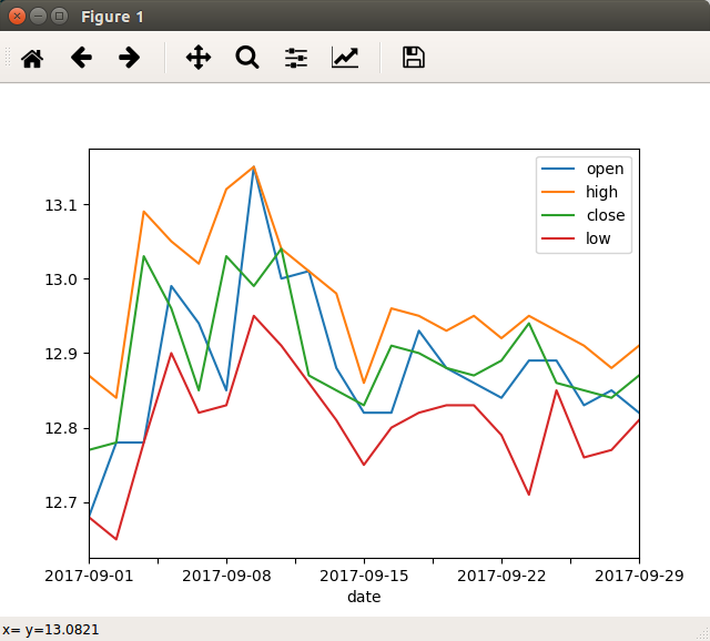
pandas生成图表
https://amaozhao.gitbooks.io/pandas-notebook/content/pandas%E4%B8%AD%E7%9A%84%E7%BB%98%E5%9B%BE%E5%87%BD%E6%95%B0.html
http://cloga.info/python/2014/02/23/plotting_with_pandas
http://blog.csdn.net/u013524655/article/details/41291715
http://blog.csdn.net/sun_shengyun/article/details/52767037
http://freefarm.cc/2016/05/24/PANDAS%E5%B8%B8%E7%94%A8%E6%89%8B%E5%86%8C-VIII-%E7%BB%98%E5%9B%BE%E5%92%8C%E5%8F%AF%E8%A7%86%E5%8C%96/
https://www.jelekinn.com/pandas-dataframe-plot.html
http://www.chenhf.com/data/pandas-done-right
http://www.cnblogs.com/splended/p/5229699.html1
2
3
4
5
6
7>>> import tushare as ts
>>> import matplotlib.pyplot as plt
>>> import pandas
>>> hist_df = ts.get_hist_data('600000', start='2017-09-01', ktype='D')
>>> new_hist_df = hist_df.sort_index(ascending=True)
>>> plot.show(new_hist_df[list(new_hist_df.columns[0:4])].plot())
pandas坑
https://tracholar.github.io/wiki/python/pandas.html
https://www.zybuluo.com/ds17/note/806790
pandas汇总统计
https://blog.csdn.net/pipisorry/article/details/256257991
2
3
4
5
6
7
8
9
10
11
12
13
14
15
16
17
18
19
20
21
22
23
24
25
26
27描述和汇总统计
方法 说明
count 非NA值的数量
describe 针对Series或各DataFrame列计算汇总统计
min,max 计算最小值和最大值
argmin,argmax 计算能够获取到最小值和最大值的索引位置(整数)
idxmin,idxmax 计算能够获取到最小值和最大值的索引值
quantile 计算样本的分位数(0到 1)
sum 值的总和
mean 值的平均数, a.mean() 默认对每一列的数据求平均值;若加上参数a.mean(1)则对每一行求平均值
media 值的算术中位数(50%分位数)
mad 根据平均值计算平均绝对离差
var 样本值的方差
std 样本值的标准差
skew 样本值的偏度(三阶矩)
kurt 样本值的峰度(四阶矩)
cumsum 样本值的累计和
cummin,cummax 样本值的累计最大值和累计最小
cumprod 样本值的累计积
diff 计算一阶差分(对时间序列很有用)
pct_change 计算百分数变化
---------------------
作者:-柚子皮-
来源:CSDN
原文:https://blog.csdn.net/pipisorry/article/details/25625799
版权声明:本文为博主原创文章,转载请附上博文链接!
Pandas速查手册中文版
https://zhuanlan.zhihu.com/p/256307001
2
3
4
5
6
7
8
9
10
11
12
13
14
15
16
17
18
19
20
21
22
23
24
25
26
27
28
29
30
31
32
33
34
35
36
37
38
39
40
41
42
43
44
45
46
47
48
49
50
51
52
53
54
55
56
57
58
59
60
61
62
63
64
65
66
67
68
69
70
71
72
73
74
75
76
77
78
79
80
81
82
83
84
85
86
87
88
89
90
91
92
93
94
95
96
97
98
99
100
101
102
103
104
105
106
107
108
109
110
111
112
113
114
115
116
117
118
119
120
121
122
123
124
125
126
127
128
129
130
131本文翻译自文章:Pandas Cheat Sheet - Python for Data Science,同时添加了部分注解。
对于数据科学家,无论是数据分析还是数据挖掘来说,Pandas是一个非常重要的Python包。它不仅提供了很多方法,使得数据处理非常简单,同时在数据处理速度上也做了很多优化,使得和Python内置方法相比时有了很大的优势。
如果你想学习Pandas,建议先看两个网站。
(1)官网:Python Data Analysis Library
(2)十分钟入门Pandas:10 Minutes to pandas
在第一次学习Pandas的过程中,你会发现你需要记忆很多的函数和方法。所以在这里我们汇总一下Pandas官方文档中比较常用的函数和方法,以方便大家记忆。同时,我们提供一个PDF版本,方便大家打印。pandas-cheat-sheet.pdf
关键缩写和包导入
在这个速查手册中,我们使用如下缩写:
df:任意的Pandas DataFrame对象
s:任意的Pandas Series对象
同时我们需要做如下的引入:
import pandas as pd
import numpy as np
导入数据
pd.read_csv(filename):从CSV文件导入数据
pd.read_table(filename):从限定分隔符的文本文件导入数据
pd.read_excel(filename):从Excel文件导入数据
pd.read_sql(query, connection_object):从SQL表/库导入数据
pd.read_json(json_string):从JSON格式的字符串导入数据
pd.read_html(url):解析URL、字符串或者HTML文件,抽取其中的tables表格
pd.read_clipboard():从你的粘贴板获取内容,并传给read_table()
pd.DataFrame(dict):从字典对象导入数据,Key是列名,Value是数据
导出数据
df.to_csv(filename):导出数据到CSV文件
df.to_excel(filename):导出数据到Excel文件
df.to_sql(table_name, connection_object):导出数据到SQL表
df.to_json(filename):以Json格式导出数据到文本文件
创建测试对象
pd.DataFrame(np.random.rand(20,5)):创建20行5列的随机数组成的DataFrame对象
pd.Series(my_list):从可迭代对象my_list创建一个Series对象
df.index = pd.date_range('1900/1/30', periods=df.shape[0]):增加一个日期索引
查看、检查数据
df.head(n):查看DataFrame对象的前n行
df.tail(n):查看DataFrame对象的最后n行
df.shape():查看行数和列数
http://df.info():查看索引、数据类型和内存信息
df.describe():查看数值型列的汇总统计
s.value_counts(dropna=False):查看Series对象的唯一值和计数
df.apply(pd.Series.value_counts):查看DataFrame对象中每一列的唯一值和计数
数据选取
df[col]:根据列名,并以Series的形式返回列
df[[col1, col2]]:以DataFrame形式返回多列
s.iloc[0]:按位置选取数据
s.loc['index_one']:按索引选取数据
df.iloc[0,:]:返回第一行
df.iloc[0,0]:返回第一列的第一个元素
数据清理
df.columns = ['a','b','c']:重命名列名
pd.isnull():检查DataFrame对象中的空值,并返回一个Boolean数组
pd.isna():检查DataFrame对象中的空值,并返回一个Boolean数组
pd.notnull():检查DataFrame对象中的非空值,并返回一个Boolean数组
df.dropna():删除所有包含空值的行
df.dropna(axis=1):删除所有包含空值的列
df.dropna(axis=1,thresh=n):删除所有小于n个非空值的行
df.fillna(x):用x替换DataFrame对象中所有的空值
s.astype(float):将Series中的数据类型更改为float类型
s.replace(1,'one'):用‘one’代替所有等于1的值
s.replace([1,3],['one','three']):用'one'代替1,用'three'代替3
df.rename(columns=lambda x: x + 1):批量更改列名
df.rename(columns={'old_name': 'new_ name'}):选择性更改列名
df.set_index('column_one'):更改索引列
df.rename(index=lambda x: x + 1):批量重命名索引
数据处理:Filter、Sort和GroupBy
df[df[col] > 0.5]:选择col列的值大于0.5的行
df.sort_values(col1):按照列col1排序数据,默认升序排列
df.sort_values(col2, ascending=False):按照列col1降序排列数据
df.sort_values([col1,col2], ascending=[True,False]):先按列col1升序排列,后按col2降序排列数据
df.groupby(col):返回一个按列col进行分组的Groupby对象
df.groupby([col1,col2]):返回一个按多列进行分组的Groupby对象
df.groupby(col1)[col2]:返回按列col1进行分组后,列col2的均值
df.pivot_table(index=col1, values=[col2,col3], aggfunc=max):创建一个按列col1进行分组,并计算col2和col3的最大值的数据透视表
df.groupby(col1).agg(np.mean):返回按列col1分组的所有列的均值
data.apply(np.mean):对DataFrame中的每一列应用函数np.mean
data.apply(np.max,axis=1):对DataFrame中的每一行应用函数np.max
数据合并
df1.append(df2):将df2中的行添加到df1的尾部
df.concat([df1, df2],axis=1):将df2中的列添加到df1的尾部
df1.join(df2,on=col1,how='inner'):对df1的列和df2的列执行SQL形式的join
数据统计
df.describe():查看数据值列的汇总统计
df.mean():返回所有列的均值
df.corr():返回列与列之间的相关系数
df.count():返回每一列中的非空值的个数
df.max():返回每一列的最大值
df.min():返回每一列的最小值
df.median():返回每一列的中位数
df.std():返回每一列的标准差
=============================================================
作者主页:笑虎(Python爱好者,关注爬虫、数据分析、数据挖掘、数据可视化等)
作者专栏主页:撸代码,学知识 - 知乎专栏
作者GitHub主页:撸代码,学知识 - GitHub